QUTCC🤗: Quantile Uncertainty Training and Conformal Calibration for Imaging Inverse Problems
Cassandra Tong Ye, Shamus Li, Tyler King, Kristina Monakhova


Abstract
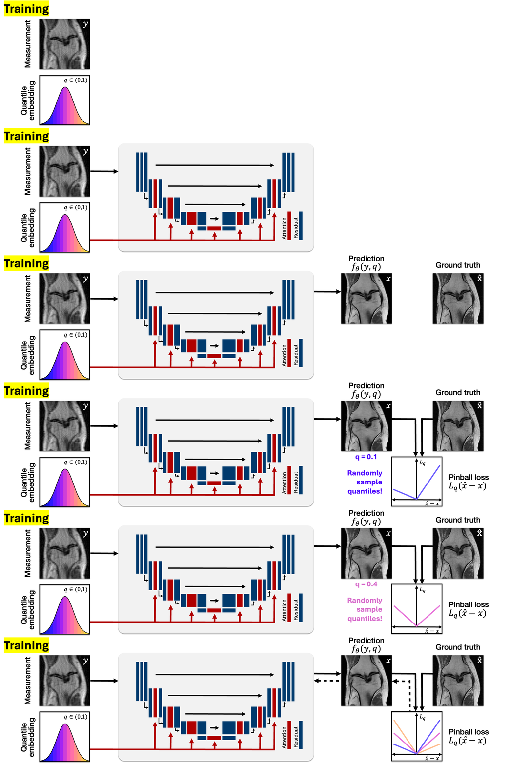
Quantile Regression: Pinball Loss
- Prior work (Im2Im-UQ) uses pinball loss to predict a fixed pair of upper and lower bounds.
- QUTCC learns the full spectrum of quantiles with a single network, known as Simultaneous Quantile Regression (SQR), applied to imaging inverse problems.
Instead of predicting a single "best guess," quantile regression predicts a chosen quantile of the target distribution, for example a value the true answer falls below 10% or 90% of the time.
- q ∈ (0, 1) is the target quantile level
- x is the true value, x̂ is the prediction
- Over- and under-estimates are penalized unequally, depending on q
Our Method: QUTCC
We propose Quantile Uncertainty Training and Conformal Calibration (QUTCC🤗), an uncertainty quantification method for imaging inverse problems.
- One learned network: a single network learns the full range of quantiles, instead of just a fixed upper and lower bound.
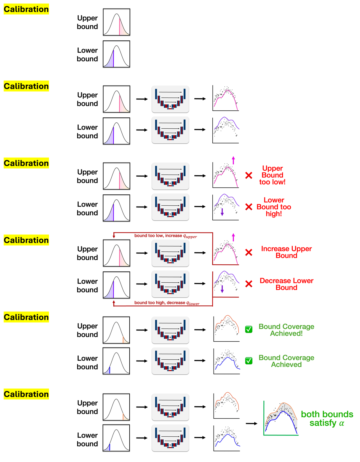
- Spatially Adaptive Calibration: bounds are scaled non-uniformly and nonlinearly during conformal calibration, instead of by one constant factor like prior methods.
- QUTCC predicts smaller UQ intervals: our method predicts tighter, more informative uncertainty intervals.
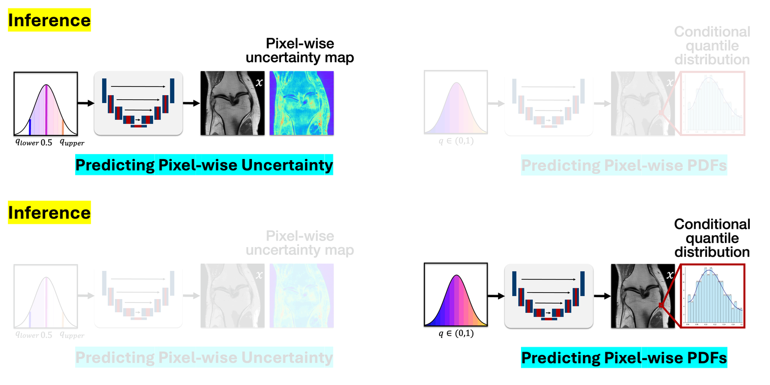
- QUTCC can predict the full conditional distribution: since every quantile is learned, QUTCC can query them all at inference time to estimate each pixel's probability distribution.
- Tested on 5 inverse problems: Gaussian noise, Poisson noise, real noise, MRI, and quantitative phase imaging (QPI).
QUTCC Produces Smaller Uncertainty Intervals
- For evaluation, we compare MC-Dropout, Deep Ensembles, Im2Im, Im2Im-Asym., K-RCPS, and our method QUTCC on five imaging inverse problems: accelerated MRI, quantitative phase imaging (QPI), and denoising under real noise, synthetic Poisson noise, and Gaussian noise.
- We compare predicted uncertainty interval lengths stratified by pixel intensity for each task, and QUTCC achieves either the smallest or second-smallest interval lengths across the tasks.
- When QUTCC ranks second, it is usually behind MC-Dropout or Deep Ensembles, which are far more costly: 28×–47× slower inference and ~10× longer training, respectively.
- QUTCC achieves the smallest mean interval length on every task among conformal methods, and remains competitive with the posterior-sampling baselines despite using a single model and only two forward passes to construct each bound.
Hover over the chart for mean ± std at each intensity. Data from Table 1 of the paper.
- QUTCC's smaller uncertainty interval lengths mean it can be more precise about pinpointing areas of error and hallucination.
- Below, we show predictions from QUTCC and Im2Im-UQ on an undersampled MRI task.
- Both models highlight regions of high uncertainty that correspond to regions of high error, but QUTCC predicts precise regions.

Pixel-wise Probability Density Functions
Because QUTCC learns every quantile, it can predict a full probability density function (PDF) at each pixel, not just an upper and lower bound.
- Prior quantile methods like Im2Im-UQ only predict discrete upper and lower bounds, so they can't describe the full distribution at a pixel.
- QUTCC queries many quantiles from a single network and calibrates them across a range of miscoverage levels α (e.g., 0.1 to 0.9).
- Together, these calibrated intervals approximate the cumulative distribution function (CDF) at each pixel. Differentiating it gives a conformalized pixel-wise PDF with coverage guarantees at each risk level.
- Below, we take a noisy Gaussian image (σ = 0.1) and compare the predicted PDFs at three pixels.
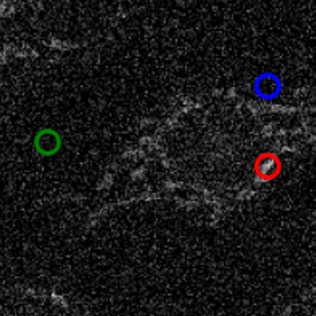
- We compare the predicted conditional PDFs of 10 representative pixels, recovered from a measurement with different levels of Gaussian and Poisson noise, across QUTCC, Ensemble, and MC-Dropout.
- Consistent with a Gaussian distribution, as σ increases, the conditional PDF at each pixel becomes broader, reflecting the increased variance of the distribution.
- In contrast, in the Poisson setting, increasing λ shifts the distribution upward, while the spread increases in proportion to the mean.
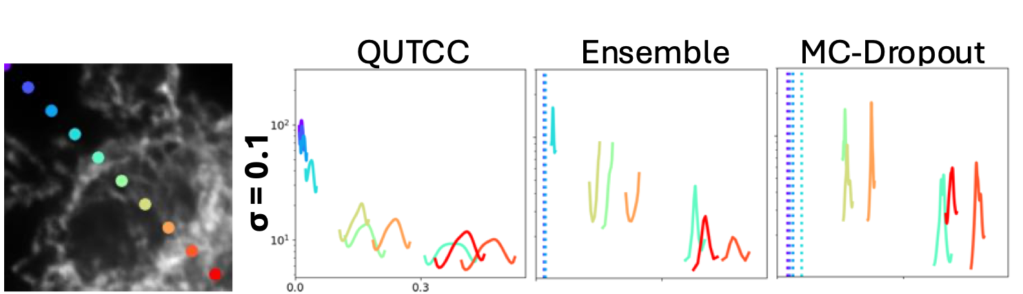
Gaussian noise, σ = 0.1. Predicted PDFs at the 10 colored pixels for QUTCC, Deep Ensemble and MC-Dropout. From Fig. 5 of the paper.